§01 · Situation
Halo Exploration needed to understand why well performance diverged.
CFrac did more than forecast. It diagnosed why performance changed.
The Halo Exploration analysis identified two major drivers of the 400% difference in production between the SW and NE part of their field: rate and landing depth.
Rate and rate timing played a signficant role in production outcome, accounting for at least 50% of the difference.
It clearly identified that as the well porpoised away from the Montney S2, CFrac fell, and as it moved toward the S2, CFrac rose.
That matters because the system is not just saying "this well will be better." It is offering an explanation of what changed in the well design and frac execution, and why the production outcome moved with it.
Commercial Takeaway
- Blind validationHalo Exploration held one reserve well back. Its six-month production was forecast from live CFrac while pumping—then compared to actual results after the job.
- Operational driversRate quality and landing depth were identified as major contributors to performance divergence.
- Future use — designDesign landing strategy before spud, and the design the pump schedule after the tops are known to maximize CFrac before the frac equipment is on location.
- Future use — operationalizeOn the day of the frac calculate CFrac in real time so you know how much oil and gas that frac will produce and compare that to your frac cost to max-min P&L.
§02 · Correlation & Validation
Cumulative CFrac tracks with production performance.
CFrac and production
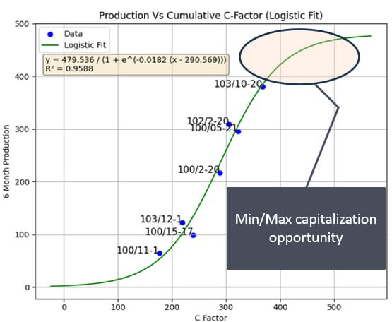
This chart is being used to support the argument that cumulative CFrac tracks with production performance. In the Halo Exploration material, 6-month production showed a statistically significant relationship with cumulative CFrac. [Confirm final public wording and exact framing.]
Correlation and validation
- Historical analysis shows strong correlation between CFrac and production.
- Higher CFrac → Higher production
- Approximate R²
The point of this work is to demonstrate that production is predicted accurately by a well's total cumulative CFrac, which is calculated by summing the final CFrac for each individual frac stage.
This is the CF-Production curve for our case study field:
y=1+e−0.0182(x−290.6)479.5
Where:
y = 6 month cumulative production,
x = cumulative CFrac per well.
In Halo Exploration's field data, cumulative CFrac was used to build a production profile and then tested against a held-back reserve well. That combination of correlation plus blind-test validation makes the proof commercially relevant.
Below, the dossier moves from correlation into why the method works, how landing depth changes the outcome, and how the same signal becomes useful for forecasting and optimization.
§03 · Why It Works
We have redefined fracture compliance for live frac operations.
We have redefined fracture compliance from its traditional pre-frac injection tests or post-ISIP leak-off to instead measure compliance the way the medical field uses it in blood vessels, a frac's ability to accept a given amount of fluid for a unit of pressure.
This framing matters because it turns compliance from a static after-the-fact concept into something that can be interpreted during pumping, when the operator still has decisions to make.
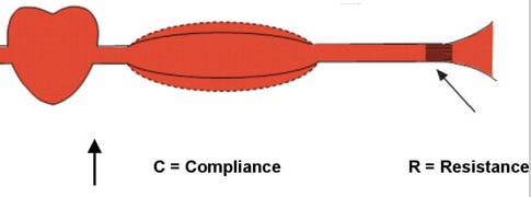
Compliance as fluid acceptance
The medical analogy is useful because it makes the concept intuitive: a more compliant system accepts more fluid for less pressure response, while a less compliant one resists it.
§04 · The Impact of Landing Depth
CFrac stage by stage analysis
For well 100/15-17, shown in dark blue, 10 stages were fracced into the Doig above the Montney. On its face that is a reasonable completion approach, but the CFrac profile shows those stages falling between 0.2 and 2.1 while the stronger fracs in the same field score between 3 and 5.
In CFrac terms, that gap matters because lower values imply the live fracture system is accepting less fluid for the fitted pressure response, which points toward lower effective permeability and smaller productive fracture area relative to the better-performing stages nearby.
For this area, a frac that does not achieve a CFrac of at least 3.1 is not economical.
AI predicted CFrac by stage
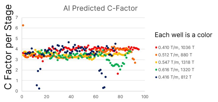
This graphic shows AI-predicted CFrac stage by stage, with each well represented by a different color. It matters because the model is not generating one abstract score per well after the fact. It is producing stage-level output that can be compared against geology, landing depth, pump behavior, and later production.
That makes CFrac useful not only for forecasting outcomes, but for diagnosing why one interval worked better than another and where the completion design or placement likely reduced value.
§05 · Landing Depth Optimization
Watching CFrac respond as the wellbore moves relative to the S2.
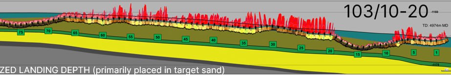
Overhead distance to the S2
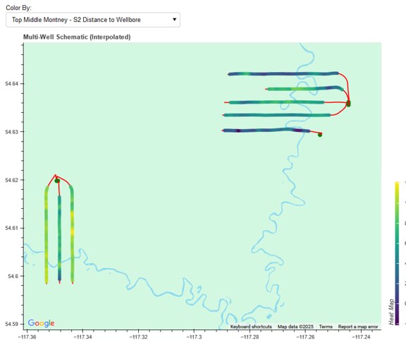
This overhead view shows well placement relative to the S2 target. Darker blue indicates intervals that remain within roughly 3 to 6 feet of the target zone, while greener intervals drift farther away, closer to 18 to 20 feet from target.
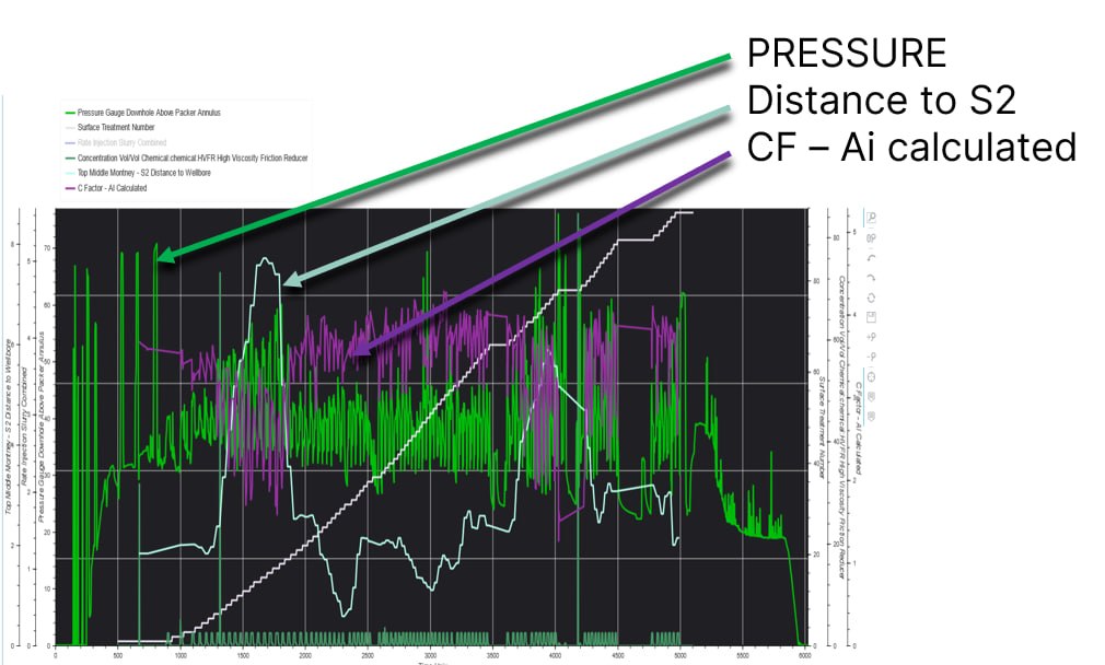
103/10-20 frac profile
This stage-by-stage frac profile shows pressure, distance to the S2, and AI-calculated CFrac moving together through the well, making the landing-depth signal visible during the frac rather than only in postmortem interpretation.
If you look at the northern most well on the over head well map you will see well 103/10-20 and you will notice the green sections of its heat map match the distance to the S2 in this his resolution frac plot
Well profile and porpoising behavior
The well profile shows when the borehole porpoises away from the S2 and when it returns. That physical movement aligns with the distance-to-S2 trend seen in the frac profile.
Why this matters
What matters here is not just that the well path moves. It is that CFrac moves with it. As the wellbore drifts away from the S2, CFrac falls. As the well returns toward the S2, CFrac rises.
That behavior is important because it shows CFrac responding to reservoir quality and pressure conditions in real time while the frac is still underway. In practical terms, it supports the claim that CFrac is measuring something physically meaningful about permeability, fracture effectiveness, and productive contact with the target interval.
This is why landing depth is not just a geosteering detail. It becomes an optimization variable that can be studied through the frac response itself.
§06 · Landing Depth & Frac Barriers
CFrac shows when the frac breaks through into better rock.
When the frac is landed more than 20 feet from the S2, it becomes separated from the target by a frac barrier. In those stages there is a distinct pressure breakdown mid-frac. Until now, that event was something engineers could observe but not confidently explain.
What matters here is what happens next: CFrac, shown in purple, rises rapidly after that pressure breakdown occurs. The interpretation is that the frac has broken through the barrier and grown into the S2, and CFrac is measuring the resulting increase in fracture area and effective permeability immediately.
Now that the event has meaning, and now that a CFrac KPI of 3.8 has been established for these wells, the frac company can be directed to continue pumping until the stage is fully stimulated. On the right-hand side, where the well is situated closer to the S2, CFrac starts higher and ends higher because the frac initiates in the S2, and there is no comparable pressure breakdown on those stages.
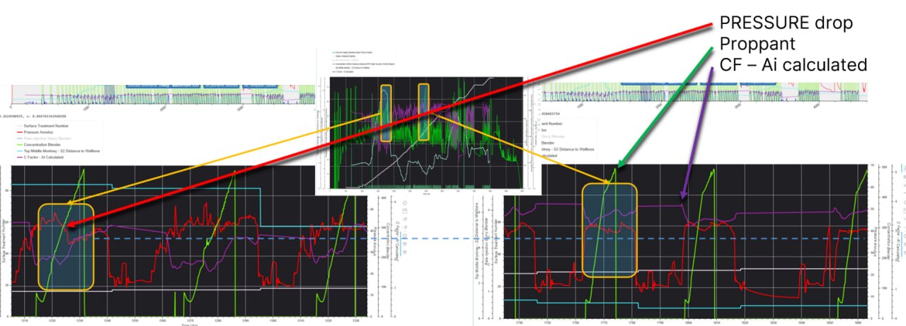
Barrier breakthrough and CFrac response
This graphic highlights the pressure break, proppant response, and AI-calculated CFrac signal that together show when the frac breaks through into higher-quality rock.
§07 · The Impact of Rate
How quickly a stage grabs rate changes how strongly it develops CFrac.
Here we zoom into the ideal section of the well where it is landed within 6 feet of the S2 and notice that three stages have been pumped differently. Two stages grab rate quickly, while the middle stage grabs rate more slowly.
The result is that the slow-rate stage starts with a lower CFrac and ends with a lower CFrac, while the stages that grab rate faster start higher and end higher.
We have seen this play out in other fields as well. That matters because it means equipment problems such as a frac blender or pump going down during a stage are no longer unknown, non-quantifiable events. We can now measure the barrels of oil and BCF lost because of frac company equipment issues.
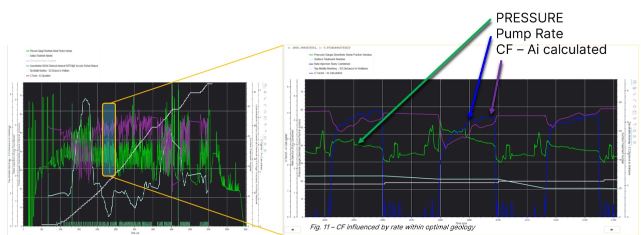
CFrac influenced by rate within optimal geology
This graphic isolates three stages in favorable geology and shows that differences in rate acquisition alone can still drive materially different CFrac outcomes.
§08 · Validation
A held-back well forecast within a few percent of six-month production.
When a held-back well forecasts within a few percent, it shows the signal is doing more than fitting old data. It is demonstrating real predictive power on wells it has not seen before.
That is the moment a technical concept becomes a commercial tool—something operators can trust in planning, budgeting, and execution.
What this validation is doing
- Production relationshipMaps total cumulative CFrac into the field production curve.
- Blind reserve wellForecast six-month production from live CFrac while pumping—on a well withheld from model training—then compare to actual results.
- Commercial meaningSupports earlier production forecasting and better-informed design/operations decisions.